Bilayer beam swelling#
Swelling of a bilayer gel beam
This is a two-dimensional plane-strain simulation
Degrees of freedom#
Displacement: u
pressure: p
chemical potential: mu
concentration: c
Units#
Length: mm
Mass: kg
Time: s
Mass density: kg/mm^3
Force: milliN
Stress: kPa
Energy: microJ
Temperature: K
Amount of substance: mol
Species concentration: mol/mm^3
Chemical potential: milliJ/mol
Molar volume: mm^3/mol
Species diffusivity: mm^2/s
Gas constant: microJ/(mol K)
Software:#
Dolfinx v0.8.0
In the collection “Example Codes for Coupled Theories in Solid Mechanics,”
By Eric M. Stewart, Shawn A. Chester, and Lallit Anand.
Import modules#
# Import FEnicSx/dolfinx
import dolfinx

# For numerical arrays
import numpy as np

# For MPI-based parallelization
from mpi4py import MPI
comm = MPI.COMM_WORLD
rank = comm.Get_rank()

# PETSc solvers
from petsc4py import PETSc

# specific functions from dolfinx modules
from dolfinx import fem, mesh, io, plot, log
from dolfinx.fem import (Constant, dirichletbc, Function, functionspace, Expression )
from dolfinx.fem.petsc import NonlinearProblem
from dolfinx.nls.petsc import NewtonSolver
from dolfinx.io import VTXWriter, XDMFFile

# specific functions from ufl modules
import ufl
from ufl import (TestFunctions, TrialFunction, Identity, grad, det, div, dev, inv, tr, sqrt, conditional ,\
                 gt, dx, inner, derivative, dot, ln, split, exp, eq, cos, sin, acos, ge, le, outer, tanh,\
                 cosh, atan, atan2)

# basix finite elements (necessary for dolfinx v0.8.0)
import basix
from basix.ufl import element, mixed_element

# Matplotlib for plotting
import matplotlib.pyplot as plt
plt.close('all')

# For timing the code
from datetime import datetime

# Set level of detail for log messages (integer)
# Guide:
# CRITICAL  = 50, // errors that may lead to data corruption
# ERROR     = 40, // things that HAVE gone wrong
# WARNING   = 30, // things that MAY go wrong later
# INFO      = 20, // information of general interest (includes solver info)
# PROGRESS  = 16, // what's happening (broadly)
# TRACE     = 13, // what's happening (in detail)
# DBG       = 10  // sundry
#
log.set_log_level(log.LogLevel.WARNING)
Define geometry#
# Create mesh
L0 = 50.0  # mm,  half-length of beam
H0 = 5.0   # mm,  height of beam

# Read in the 2D mesh and cell tags
with XDMFFile(MPI.COMM_WORLD,"meshes/bilayer_beam.xdmf",'r') as infile:
    domain = infile.read_mesh(name="Grid",xpath="/Xdmf/Domain")
    cell_tags = infile.read_meshtags(domain,name="Grid")
domain.topology.create_connectivity(domain.topology.dim, domain.topology.dim-1)

# Also read in 1D facets for applying BCs
with XDMFFile(MPI.COMM_WORLD,"meshes/facet_bilayer_beam.xdmf",'r') as infile:
    facet_tags = infile.read_meshtags(domain,name="Grid")

# A single point for "grounding" the displacement and phi
def ground(x):
    return np.logical_and(np.isclose(x[0], 0), np.isclose(x[1], 0))

x = ufl.SpatialCoordinate(domain)
Print out the unique cell number indices
top_imap = domain.topology.index_map(2)      # index map of 2D entities in domain
values = np.zeros(top_imap.size_global)      # an array of zeros of the same size as number of 2D entities
values[cell_tags.indices]=cell_tags.values   # populating the array with facet tag index numbers
print(np.unique(cell_tags.values))           # printing the unique indices

# # Markers from gmsh
# - "Bottom_layer", 13
# - "Top_layer", 14
[13 14]
Print out the unique facet index numbers
top_imap = domain.topology.index_map(1)      # index map of 1D entities in domain
values = np.zeros(top_imap.size_global)      # an array of zeros of the same size as number of 2D entities
values[facet_tags.indices]=facet_tags.values # populating the array with facet tag index numbers
print(np.unique(facet_tags.values))          # printing the unique

# # Markers from gmsh
# - "Left_edge", 8
# - "Bottom_edge", 9
# - "Right_edge", 10
# - "Top_edge", 11
# - "Middle_edge", 12
[ 8 9 10 11 12]
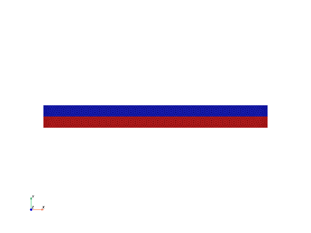
Visualize reference configuration
import pyvista
pyvista.set_jupyter_backend('html')
from dolfinx.plot import vtk_mesh
pyvista.start_xvfb()

# initialize a plotter
plotter = pyvista.Plotter()

# Add the mesh.
topology, cell_types, geometry = plot.vtk_mesh(domain, domain.topology.dim)
grid = pyvista.UnstructuredGrid(topology, cell_types, geometry)
plotter.add_mesh(grid, show_edges=True, opacity=0.25)

# Add colored 2D surfaces for the named surfaces
bottom_surf = pyvista.UnstructuredGrid(*vtk_mesh(domain, domain.topology.dim,cell_tags.indices[cell_tags.values==13]) )
top_surf = pyvista.UnstructuredGrid(*vtk_mesh(domain, domain.topology.dim,cell_tags.indices[cell_tags.values==14]) )
#
actor = plotter.add_mesh(bottom_surf, show_edges=False,color="red")  # bottom layer is red
actor2 = plotter.add_mesh(top_surf,   show_edges=False,color="blue") #  top  layer is blue

plotter.view_xy()

#labels = dict(zlabel='Z', xlabel='X', ylabel='Y')
labels = dict(xlabel='X', ylabel='Y')
plotter.add_axes(**labels)

plotter.screenshot("results/beam_mesh.png")

from IPython.display import Image
Image(filename='results/beam_mesh.png')

# # Use the following  commands for a  zoom-able  view
# if not pyvista.OFF_SCREEN:
#     plotter.show()
# else:
#     plotter.screenshot("beam_mesh.png")
Define boundary and volume integration measure#
# Define the boundary integration measure "ds" using the facet tags,
# also specify the number of surface quadrature points.
ds = ufl.Measure('ds', domain=domain, subdomain_data=facet_tags, metadata={'quadrature_degree':2})

# Define the volume integration measure "dx"
# also specify the number of volume quadrature points.
dx = ufl.Measure('dx', domain=domain, metadata={'quadrature_degree': 2})

# Create facet to cell connectivity required to determine boundary facets.
domain.topology.create_connectivity(domain.topology.dim, domain.topology.dim)
domain.topology.create_connectivity(domain.topology.dim, domain.topology.dim-1)
domain.topology.create_connectivity(domain.topology.dim-1, domain.topology.dim)

# #  Define facet normal
n2D = ufl.FacetNormal(domain)
n = ufl.as_vector([n2D[0], n2D[1], 0.0]) # define n as a 3D vector for later use
Material parmeters#
# A function for constructing spatially varying (piecewise-constant) material parameters

# Need some extra infrastructure for the spatially-discontinuous material property fields
Vmat = functionspace(domain, ("DG", 0)) # create a DG0 function space on the domain

# Define function ``mat'' for assigning different values for material properties
# for the bottom and top layers
#
def mat(prop_val_bottom, prop_val_top):

    # Define an empty "prop" material parameter function,
    # which lives on the DG0 function space.
    prop = Function(Vmat)

    # Now, actualy assign the desired values of the material properies to the new field.
    #
    coords = Vmat.tabulate_dof_coordinates()
    #
    # loop over the coordinates and assign the relevant material property,
    # based on the local cell tag number.
    for i in range(coords.shape[0]):
        if cell_tags.values[i] == 13:
            prop.vector.setValueLocal(i, prop_val_bottom)
        elif cell_tags.values[i] == 14:
            prop.vector.setValueLocal(i, prop_val_top)

        # else:
        #     prop.vector.setValueLocal(i, prop_val_top)

    return prop
# Set the locking stretch to a large number to model a Neo-Hookean material
#
Gshear_0= mat(50000,1000)                                    # Shear moduluii for the two layers
lambdaL = Constant(domain,PETSc.ScalarType(100))             # Locking stretch, Neo_hookean material
Kbulk   = Constant(domain,PETSc.ScalarType(1.E6))            # Bulk modulus, kPa
Omega   = Constant(domain,PETSc.ScalarType(1.00e5))          # Molar volume of fluid
D       = Constant(domain,PETSc.ScalarType(5.00e-3))         # Diffusivity
chi     = mat(0.9,0.1)                                       # Flory-Huggins chi parameter for the two layers
theta0  = Constant(domain,PETSc.ScalarType(298) )            # Reference temperature
R_gas   = Constant(domain,PETSc.ScalarType(8.3145e6))        # Gas constant
RT      = Constant(domain,PETSc.ScalarType(8.3145e6*theta0))
#
phi0    = Constant(domain,PETSc.ScalarType(0.999))                # Initial polymer volume fraction
mu0     = Constant(domain,PETSc.ScalarType(ln(1.0-phi0) + phi0 )) # Initial chemical potential
c0      = Constant(domain,PETSc.ScalarType((1/phi0) - 1))         # Initial concentration
pyvista.set_jupyter_backend('html')
pyvista.start_xvfb()
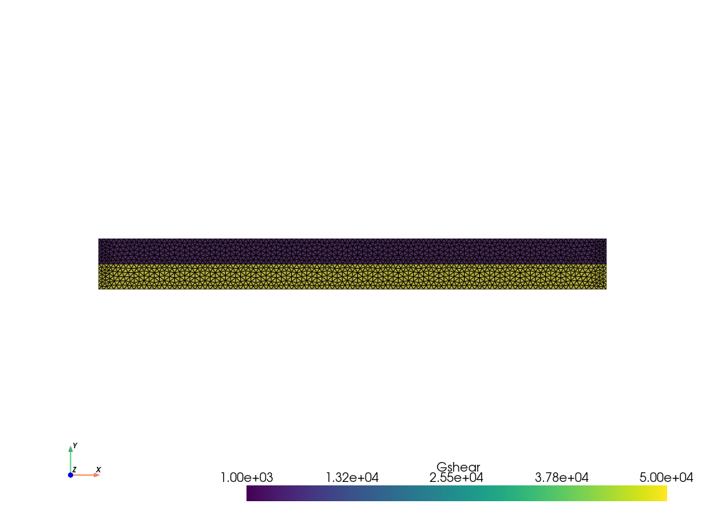
# Prepare the gshear field for plotting
V = functionspace(domain,("DG",1)) # for some reason, we need a degree 1 DG function space in order to plot in Pyvista.
vtkdata = vtk_mesh(V)
grid = pyvista.UnstructuredGrid(*vtkdata)
#
grid["Gshear"] = Gshear_0.x.array # interpolate the Gshear_0 data onto the DG1 space.
#
grid.set_active_scalars("Gshear")
actor = plotter.add_mesh(grid, show_edges=True) # plot Gshear_0 values.
# turn the camera around so that the inclusion is visible
plotter.camera.azimuth = 180.0
plotter.view_xy()
#labels = dict(xlabel='X', ylabel='Y',zlabel='Z')
labels = dict(xlabel='X', ylabel='Y')
plotter.add_axes(**labels)
plotter.screenshot("results/bilayer_shear_moduli.png")
from IPython.display import Image
Image(filename='results/bilayer_shear_moduli.png')
# if not pyvista.OFF_SCREEN:
# plotter.show()
# else:
# plotter.screenshot("results/bilayer_shear_moduli.png")
Function spaces#
# Define function space, both vectorial and scalar
#
U2 = element("Lagrange", domain.basix_cell(), 2, shape=(2,)) # For displacement
P1 = element("Lagrange", domain.basix_cell(), 1) # For pressure, chemical potential and  species concentration
#
TH = mixed_element([U2, P1, P1, P1])  # Taylor-Hood style mixed element
ME = functionspace(domain, TH)        # Total space for all DOFs

# Define actual functions with the required DOFs
w = Function(ME)
u, p, mu, c = split(w)  # displacement u, pressure p, chemical potential mu, and concentration c

# A copy of functions to store values in the previous step for time-stepping
w_old = Function(ME)
u_old,  p_old, mu_old, c_old = split(w_old)

# Define test functions
u_test, p_test,  mu_test, c_test = TestFunctions(ME)

# Define trial functions needed for automatic differentiation
dw = TrialFunction(ME)
Initial conditions#
The initial conditions for \(\mathbf{u}\) and \(p\) are zero everywhere.
These are imposed automatically, since we have not specified any non-zero initial conditions.
We do, however, need to impose the uniform initial conditions for \(\mu=\mu_0\) and \(\hat{c} = \hat{c}_0\) which correspond to \(\phi_0 = 0.999\). This is done below.
# Assign initial  normalized chemical potential  mu0 to the domain
w.sub(2).interpolate(lambda x: np.full((x.shape[1],),  mu0))
w_old.sub(2).interpolate(lambda x: np.full((x.shape[1],), mu0))

# Assign initial  value of normalized concentration  c0 to the domain
c0 = Constant(domain,PETSc.ScalarType((1/phi0) - 1)) # initial concentration
#
w.sub(3).interpolate(lambda x: np.full((x.shape[1],),  c0))
w_old.sub(3).interpolate(lambda x: np.full((x.shape[1],), c0))
Subroutines for kinematics and constitutive equations#
# Special gradient operators for plane strain
#
# Gradient of vector field u
def pe_grad_vector(u):

    grad_u = grad(u)

    pe_grad_u = ufl.as_tensor([ [grad_u[0,0], grad_u[0,1], 0.0],
                                [grad_u[1,0], grad_u[1,1], 0.0],
                                [        0.0,         0.0, 0.0] ])
    return pe_grad_u

# Gradient of scalar field y
# (just need an extra zero for dimensions to work out)
def pe_grad_scalar(y):

    grad_y = grad(y)

    pe_grad_y = ufl.as_vector([grad_y[0], grad_y[1], 0.0])

    return pe_grad_y

# Plane strain deformation gradient
def F_pe_calc(u):

    dim = len(u)                # dimension of problem (2)

    Id = Identity(dim)          # 2D Identity tensor

    F = Id + grad(u)            # 2D Deformation gradient

    F_pe =  ufl.as_tensor([ [F[0,0], F[0,1], 0.0],
                            [F[1,0], F[1,1], 0.0],
                            [   0.0,    0.0, 1.0] ]) # Full plane strain F
    return F_pe

def lambdaBar_calc(u):
    F = F_pe_calc(u)
    C = F.T*F
    Cdis = J**(-2/3)*C
    I1 = tr(Cdis)
    lambdaBar = sqrt(I1/3.0)
    return lambdaBar

#---------------------------------------------------
# Calculate zeta
#---------------------------------------------------
def zeta_calc(u):
    lambdaBar = lambdaBar_calc(u)
    # Use Pade approximation of Langevin inverse
    z    = lambdaBar/lambdaL
    z    = conditional(gt(z,0.95), 0.95, z) # Keep simulation from blowing up
    beta = z*(3.0 - z**2.0)/(1.0 - z**2.0)
    zeta = (lambdaL/(3*lambdaBar))*beta
    return zeta

#---------------------------------------------------
# Calculate zeta0
#---------------------------------------------------
def zeta0_calc():
    # Use Pade approximation of Langevin inverse (A. Cohen, 1991)
    z    = 1/lambdaL
    z    = conditional(gt(z,0.95), 0.95, z) # Keep from blowing up
    beta0 = z*(3.0 - z**2.0)/(1.0 - z**2.0)
    zeta0 = (lambdaL/3)*beta0
    return zeta0

#---------------------------------------------------
# Subroutine for calculating the elastic jacobian Je
#---------------------------------------------------
def Je_calc(u,c):
    F = F_pe_calc(u)
    detF = det(F)
    #
    detFs = 1.0 + c          # = Js
    Je    = (detF/detFs)     # = Je
    return   Je

#----------------------------------------------
# Subroutine for calculating the Piola  stress
#----------------------------------------------
def Piola_calc(u,p):
    F     = F_pe_calc(u)
    zeta  = zeta_calc(u)
    zeta0 = zeta0_calc()
    Piola = (zeta*F - zeta0*inv(F.T) ) - J*p*inv(F.T)/Gshear_0
    return Piola

#--------------------------------------------------------------
# Subroutine for calculating the normalized species flux
#--------------------------------------------------------------
def Flux_calc(u, mu, c):
    F = F_pe_calc(u)
    #
    Cinv = inv(F.T*F)
    #
    Mob = (D*c)/(Omega*RT)*Cinv
    #
    Jmat = - RT* Mob * grad(mu)
    return Jmat
Evaluate kinematics and constitutive relations#
# Kinematics
F = F_pe_calc(u)
J = det(F)  # Total volumetric jacobian
#
lambdaBar = lambdaBar_calc(u)
#
# Elastic volumetric Jacobian
Je     = Je_calc(u,c)
Je_old = Je_calc(u_old,c_old)

#  Normalized Piola stress
Piola = Piola_calc(u, p)

#  Normalized species  flux
Jmat = Flux_calc(u, mu, c)
Weak forms#
# Residuals:
# Res_0: Balance of forces (test fxn: u)
# Res_1: Pressure variable (test fxn: p)
# Res_2: Balance of mass   (test fxn: mu)
# Res_3: Auxiliary variable (test fxn: c)

# Time step field, constant within body
dk = Constant(domain, PETSc.ScalarType(dt))

# The weak form for the equilibrium equation
Res_0 = inner(Piola , pe_grad_vector(u_test) )*dx

# The weak form for the auxiliary pressure variable
Res_1 = dot((p*Je/Kbulk + ln(Je)) , p_test)*dx

# The weak form for the mass balance of solvent
Res_2 = dot((c - c_old)/dk, mu_test)*dx \
        -  Omega*dot(Jmat , pe_grad_scalar(mu_test) )*dx

# The weak form for the concentration
fac = 1/(1+c)
fac1 =  mu - ( ln(1.0-fac)+ fac + chi*fac*fac)
fac2 = - (Omega*Je/RT)*p
fac3 = - (1./2.) * (Omega/(Kbulk*RT)) * ((p*Je)**2.0) # This works
fac4 = fac1 + fac2 + fac3
#
Res_3 = dot(fac4, c_test)*dx

# Total weak form
Res = Res_0 + Res_1 + Res_2 + Res_3

# Automatic differentiation tangent:
a = derivative(Res, w, dw)
Set-up output files#
# results file name
results_name = "gel_pe_bilayer_beam"

# Function space for projection of results
U1 = element("DG", domain.basix_cell(), 1, shape=(2,))  # For displacement
P0 = element("DG", domain.basix_cell(), 1)              # For  pressure, chemical potential, and concentration
T1 = element("DG", domain.basix_cell(), 1, shape=(3,3)) # For stress tensor

V1 = fem.functionspace(domain, P0) # Scalar function space
V2 = fem.functionspace(domain, U1) # Vector function space
V3 = fem.functionspace(domain, T1) # Tensor function space

# basic fields to write to output file
u_vis = Function(V2)
u_vis.name = "disp"

p_vis = Function(V1)
p_vis.name = "p"

mu_vis = Function(V1)
mu_vis.name = "mu"

c_vis = Function(V1)
c_vis.name = "c"

# calculated fields to write to output file
phi = 1/(1+c)
phi_vis = Function(V1)
phi_vis.name = "phi"
phi_expr = Expression(phi,V1.element.interpolation_points())

J_vis = Function(V1)
J_vis.name = "J"
J_expr = Expression(J,V1.element.interpolation_points())

lambdaBar_vis = Function(V1)
lambdaBar_vis.name = "lambdaBar"
lambdaBar_expr = Expression(lambdaBar,V1.element.interpolation_points())

P11 = Function(V1)
P11.name = "P11"
P11_expr = Expression(Piola[0,0],V1.element.interpolation_points())
#
P22 = Function(V1)
P22.name = "P22"
P22_expr = Expression(Piola[1,1],V1.element.interpolation_points())
#
P33 = Function(V1)
P33.name = "P33"
P33_expr = Expression(Piola[2,2],V1.element.interpolation_points())

# Mises stress
T   = Piola*F.T/J
T0   = T - (1/3)*tr(T)*Identity(3)
Mises = sqrt((3/2)*inner(T0, T0))
Mises_vis= Function(V1,name="Mises")
Mises_expr = Expression(Mises,V1.element.interpolation_points())

# set up the output VTX files.
file_results = VTXWriter(
    MPI.COMM_WORLD,
    "results/" + results_name + ".bp",
    [  # put the functions here you wish to write to output
        u_vis, p_vis, mu_vis, c_vis, phi_vis, J_vis, P11, P22, P33,
        lambdaBar_vis,Mises_vis,
    ],
    engine="BP4",
)

def writeResults(t):
       # Output field interpolation
       u_vis.interpolate(w.sub(0))
       p_vis.interpolate(w.sub(1))
       mu_vis.interpolate(w.sub(2))
       c_vis.interpolate(w.sub(3))
       phi_vis.interpolate(phi_expr)
       J_vis.interpolate(J_expr)
       P11.interpolate(P11_expr)
       P22.interpolate(P22_expr)
       P33.interpolate(P33_expr)
       lambdaBar_vis.interpolate(lambdaBar_expr)
       Mises_vis.interpolate(Mises_expr)

       # Write output fields
       file_results.write(t)
Infrastructure for pulling out time history data (dispalcement, force, etc.)#
# Identify point for reporting dislacement
pointForDisp = np.array([L0,H0/2,0.0])

bb_tree = dolfinx.geometry.bb_tree(domain,domain.topology.dim)
cell_candidates = dolfinx.geometry.compute_collisions_points(bb_tree, pointForDisp)
colliding_cells = dolfinx.geometry.compute_colliding_cells(domain, cell_candidates, pointForDisp).array
Analysis Step#
# Give the step a descriptive name
step = "Swell"
Boundary conditions#
# # Markers from gmsh
# - "Left_edge", 8
# - "Bottom_edge", 9
# - "Right_edge", 10
# - "Top_edge", 11
# - "Middle_edge", 12

# Constant for applied  chemical potential
mu_cons = Constant(domain,PETSc.ScalarType(muRamp(0)))

# Find the specific DOFs which will be constrained.
Left_u1_dofs = fem.locate_dofs_topological(ME.sub(0).sub(0), facet_tags.dim, facet_tags.find(8))
#
Top_mu_dofs  = fem.locate_dofs_topological(ME.sub(2), facet_tags.dim, facet_tags.find(11))

# building Dirichlet BCs
bcs_1 = dirichletbc(0.0, Left_u1_dofs, ME.sub(0).sub(0))   # u1 fix Left
#
bcs_2 = dirichletbc(mu_cons, Top_mu_dofs, ME.sub(2))       # mu_cons- Top

# Zero displacement bc for left bottom node
V0, submap = ME.sub(0).collapse()
fixed_u_dofs = fem.locate_dofs_geometrical((ME.sub(0), V0), ground)
fixed_disp = Function(V0)
fixed_disp.interpolate(lambda x: np.stack(( np.zeros(x.shape[1]), np.zeros(x.shape[1]) ) ) )
#
bcs_3 = dirichletbc(fixed_disp, fixed_u_dofs, ME.sub(0))        # u fix -  bottom left node

bcs = [bcs_1, bcs_2, bcs_3]
Define the nonlinear variational problem#
# Set up nonlinear problem
problem = NonlinearProblem(Res, w, bcs, a)

# The global newton solver and params
solver = NewtonSolver(MPI.COMM_WORLD, problem)
solver.convergence_criterion = "incremental"
solver.rtol = 1e-8
solver.atol = 1e-8
solver.max_it = 50
solver.report = True

#  The Krylov solver parameters.
ksp = solver.krylov_solver
opts = PETSc.Options()
option_prefix = ksp.getOptionsPrefix()
opts[f"{option_prefix}ksp_type"] = "preonly"
opts[f"{option_prefix}pc_type"] = "lu" # do not use 'gamg' pre-conditioner
opts[f"{option_prefix}pc_factor_mat_solver_type"] = "mumps"
opts[f"{option_prefix}ksp_max_it"] = 30
ksp.setFromOptions()
Initialize arrays for storing output history#
# Arrays for storing output history
totSteps = 100000
timeHist0 = np.zeros(shape=[totSteps])
timeHist1 = np.zeros(shape=[totSteps])
# timeHist2 = np.zeros(shape=[totSteps])
# timeHist3 = np.zeros(shape=[totSteps])
# #
# timeHist3[0] = mu0 # Initialize the chemical potential

# Initialize a counter for reporting data
ii = 0

# Write initial state to file
writeResults(t=0.0)
Start calculation loop#
# Print  message for simulation start
print("------------------------------------")
print("Simulation Start")
print("------------------------------------")
# Store start time
startTime = datetime.now()

# Time-stepping solution procedure loop
while (round(t + dt, 9) <= Ttot):

    # increment time
    t += dt
    # increment counter
    ii += 1

    # update time variables in time-dependent BCs
    mu_cons.value = float(muRamp(t))

    # Solve the problem
    try:
        (iter, converged) = solver.solve(w)
    except: # Break the loop if solver fails
        print("Ended Early")
        break

    # Collect results from MPI ghost processes
    w.x.scatter_forward()

    # Write output to file
    writeResults(t)

    # Update DOFs for next step
    w_old.x.array[:] = w.x.array


    # Store  displacement at a particular point  at this time
    #
    timeHist0[ii] = t                                                        # time
    #
    timeHist1[ii] = w.sub(0).sub(1).eval([L0,H0/2,0.0],colliding_cells[0])[0] # displacement of tip of beam

    # Print progress of calculation
    if ii%1 == 0:
        now = datetime.now()
        current_time = now.strftime("%H:%M:%S")
        print("Step: {} | Increment: {}, Iterations: {}".\
              format(step, ii, iter))
        print("      Simulation Time: {} s  of  {} s".\
              format(round(t,4), Ttot))
        print()

# close the output file.
file_results.close()

# End analysis
print("-----------------------------------------")
print("End computation")
# Report elapsed real time for the analysis
endTime = datetime.now()
elapseTime = endTime - startTime
print("------------------------------------------")
print("Elapsed real time:  {}".format(elapseTime))
print("------------------------------------------")
------------------------------------
Simulation Start
------------------------------------
Step: Swell | Increment: 1, Iterations: 4
      Simulation Time: 20.0 s  of  1300 s

Step: Swell | Increment: 2, Iterations: 5
      Simulation Time: 40.0 s  of  1300 s

Step: Swell | Increment: 3, Iterations: 5
      Simulation Time: 60.0 s  of  1300 s

Step: Swell | Increment: 4, Iterations: 5
      Simulation Time: 80.0 s  of  1300 s

Step: Swell | Increment: 5, Iterations: 5
      Simulation Time: 100.0 s  of  1300 s

Step: Swell | Increment: 6, Iterations: 5
      Simulation Time: 120.0 s  of  1300 s

Step: Swell | Increment: 7, Iterations: 5
      Simulation Time: 140.0 s  of  1300 s

Step: Swell | Increment: 8, Iterations: 5
      Simulation Time: 160.0 s  of  1300 s

Step: Swell | Increment: 9, Iterations: 5
      Simulation Time: 180.0 s  of  1300 s

Step: Swell | Increment: 10, Iterations: 5
      Simulation Time: 200.0 s  of  1300 s

Step: Swell | Increment: 11, Iterations: 5
      Simulation Time: 220.0 s  of  1300 s

Step: Swell | Increment: 12, Iterations: 5
      Simulation Time: 240.0 s  of  1300 s

Step: Swell | Increment: 13, Iterations: 5
      Simulation Time: 260.0 s  of  1300 s

Step: Swell | Increment: 14, Iterations: 5
      Simulation Time: 280.0 s  of  1300 s

Step: Swell | Increment: 15, Iterations: 5
      Simulation Time: 300.0 s  of  1300 s

Step: Swell | Increment: 16, Iterations: 5
      Simulation Time: 320.0 s  of  1300 s

Step: Swell | Increment: 17, Iterations: 5
      Simulation Time: 340.0 s  of  1300 s

Step: Swell | Increment: 18, Iterations: 5
      Simulation Time: 360.0 s  of  1300 s

Step: Swell | Increment: 19, Iterations: 5
      Simulation Time: 380.0 s  of  1300 s

Step: Swell | Increment: 20, Iterations: 5
      Simulation Time: 400.0 s  of  1300 s

Step: Swell | Increment: 21, Iterations: 5
      Simulation Time: 420.0 s  of  1300 s

Step: Swell | Increment: 22, Iterations: 5
      Simulation Time: 440.0 s  of  1300 s

Step: Swell | Increment: 23, Iterations: 5
      Simulation Time: 460.0 s  of  1300 s

Step: Swell | Increment: 24, Iterations: 5
      Simulation Time: 480.0 s  of  1300 s

Step: Swell | Increment: 25, Iterations: 5
      Simulation Time: 500.0 s  of  1300 s

Step: Swell | Increment: 26, Iterations: 5
      Simulation Time: 520.0 s  of  1300 s

Step: Swell | Increment: 27, Iterations: 5
      Simulation Time: 540.0 s  of  1300 s

Step: Swell | Increment: 28, Iterations: 5
      Simulation Time: 560.0 s  of  1300 s

Step: Swell | Increment: 29, Iterations: 5
      Simulation Time: 580.0 s  of  1300 s

Step: Swell | Increment: 30, Iterations: 5
      Simulation Time: 600.0 s  of  1300 s

Step: Swell | Increment: 31, Iterations: 5
      Simulation Time: 620.0 s  of  1300 s

Step: Swell | Increment: 32, Iterations: 5
      Simulation Time: 640.0 s  of  1300 s

Step: Swell | Increment: 33, Iterations: 5
      Simulation Time: 660.0 s  of  1300 s

Step: Swell | Increment: 34, Iterations: 5
      Simulation Time: 680.0 s  of  1300 s

Step: Swell | Increment: 35, Iterations: 5
      Simulation Time: 700.0 s  of  1300 s

Step: Swell | Increment: 36, Iterations: 5
      Simulation Time: 720.0 s  of  1300 s

Step: Swell | Increment: 37, Iterations: 5
      Simulation Time: 740.0 s  of  1300 s

Step: Swell | Increment: 38, Iterations: 5
      Simulation Time: 760.0 s  of  1300 s

Step: Swell | Increment: 39, Iterations: 5
      Simulation Time: 780.0 s  of  1300 s

Step: Swell | Increment: 40, Iterations: 5
      Simulation Time: 800.0 s  of  1300 s

Step: Swell | Increment: 41, Iterations: 5
      Simulation Time: 820.0 s  of  1300 s

Step: Swell | Increment: 42, Iterations: 5
      Simulation Time: 840.0 s  of  1300 s

Step: Swell | Increment: 43, Iterations: 5
      Simulation Time: 860.0 s  of  1300 s

Step: Swell | Increment: 44, Iterations: 5
      Simulation Time: 880.0 s  of  1300 s

Step: Swell | Increment: 45, Iterations: 5
      Simulation Time: 900.0 s  of  1300 s

Step: Swell | Increment: 46, Iterations: 5
      Simulation Time: 920.0 s  of  1300 s

Step: Swell | Increment: 47, Iterations: 5
      Simulation Time: 940.0 s  of  1300 s

Step: Swell | Increment: 48, Iterations: 5
      Simulation Time: 960.0 s  of  1300 s

Step: Swell | Increment: 49, Iterations: 5
      Simulation Time: 980.0 s  of  1300 s

Step: Swell | Increment: 50, Iterations: 5
      Simulation Time: 1000.0 s  of  1300 s

Step: Swell | Increment: 51, Iterations: 5
      Simulation Time: 1020.0 s  of  1300 s

Step: Swell | Increment: 52, Iterations: 5
      Simulation Time: 1040.0 s  of  1300 s

Step: Swell | Increment: 53, Iterations: 5
      Simulation Time: 1060.0 s  of  1300 s

Step: Swell | Increment: 54, Iterations: 5
      Simulation Time: 1080.0 s  of  1300 s

Step: Swell | Increment: 55, Iterations: 5
      Simulation Time: 1100.0 s  of  1300 s

Step: Swell | Increment: 56, Iterations: 5
      Simulation Time: 1120.0 s  of  1300 s

Step: Swell | Increment: 57, Iterations: 5
      Simulation Time: 1140.0 s  of  1300 s

Step: Swell | Increment: 58, Iterations: 5
      Simulation Time: 1160.0 s  of  1300 s

Step: Swell | Increment: 59, Iterations: 5
      Simulation Time: 1180.0 s  of  1300 s

Step: Swell | Increment: 60, Iterations: 5
      Simulation Time: 1200.0 s  of  1300 s

Step: Swell | Increment: 61, Iterations: 5
      Simulation Time: 1220.0 s  of  1300 s

Step: Swell | Increment: 62, Iterations: 5
      Simulation Time: 1240.0 s  of  1300 s

Step: Swell | Increment: 63, Iterations: 5
      Simulation Time: 1260.0 s  of  1300 s

Step: Swell | Increment: 64, Iterations: 5
      Simulation Time: 1280.0 s  of  1300 s

Step: Swell | Increment: 65, Iterations: 5
      Simulation Time: 1300.0 s  of  1300 s

-----------------------------------------
End computation
------------------------------------------
Elapsed real time:  0:00:16.047489
------------------------------------------
Plot results#
# Set up font size, initialize colors array
font = {'size' : 14}
plt.rc('font', **font)
#
prop_cycle = plt.rcParams['axes.prop_cycle']
colors = prop_cycle.by_key()['color']
# Only plot as far as we have time history data
ind = np.argmax(timeHist0[:])
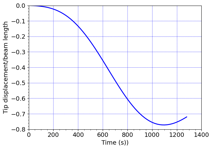
# Create figure for temperature versus tip-displacement curve.
#
fig = plt.figure()
ax=fig.gca()
#---------------------------------------------------------------------------------------------
plt.plot(timeHist0[0:ind], timeHist1[0:ind]/L0, c='b', linewidth=2.0)
#---------------------------------------------------------------------------------------------
plt.xlim(0,1400)
plt.ylim(-0.8,0.0)
#
plt.grid(linestyle="--", linewidth=0.5, color='b')
# ax.set_ylabel("Surface temperature change, K",size=14)
ax.set_xlabel("Time (s))",size=14)
ax.set_ylabel(r'Tip displacement/beam length',size=14)
#ax.set_title(r'Temperature versus tip displacement curve', size=14, weight='normal')
#
from matplotlib.ticker import AutoMinorLocator,FormatStrFormatter
ax.xaxis.set_minor_locator(AutoMinorLocator())
ax.yaxis.set_minor_locator(AutoMinorLocator())
#plt.legend()
import matplotlib.ticker as ticker
ax.xaxis.set_major_formatter(ticker.FormatStrFormatter('%0.0f'))
# Save figure
fig = plt.gcf()
fig.set_size_inches(7,5)
plt.tight_layout()
plt.savefig("results/gel_pe_bilayer_tip_displacement.png", dpi=600)